
Improvements to the Distribution & Braid Algorithm in PacMaze
This article illustrates how the Distribution Algorithm and Braid Algorithm by Ioannidis (2016) are improved in PacMaze.
Readers should know about the PacMaze project before reading this article.
读者在阅读本文前,应当先了解 PacMaze 项目。
Improvements to the Distribution Algorithm
The original Distribution Algorithm is simply an algorithm that combines random numbers with probability judgement logic. In order to achieve the desired effect of the optimisation, it is necessary to understand what kind of wall layout provides better game experience than random generation.
Figure 1 shows the “classic” map that comes with the PacMaze game. This is the map that is created by default when the player creates a new map in the “Edit Maps” page (the player can then modify the map based on it). The wall layout design of this map takes some inspiration from the famous Pac-Man game (Namco, 1980) map. It has been tested to some extent and has playability and some challenge.
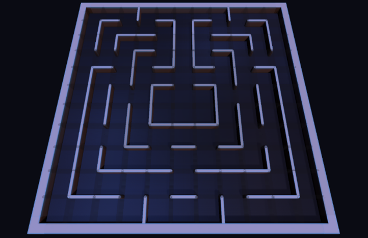
Figure 2 shows the number of neighbours for every tile in this classic map. Different numbers of neighbours are marked in different colours to improve intuition.
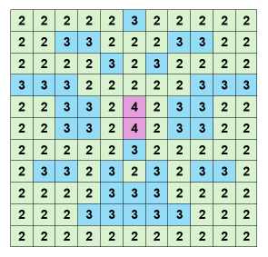
From Figure 2, it is possible to detect a certain degree of regularity in the wall layouts that are more suitable for being used as PacMaze game maps. It can be concluded by the following four patterns:
- The outermost ring should have a fairly small number of tiles with 3 neighbours and the vast majority of tiles should have only 2 neighbours. This is because the outermost ring should play less of a “traffic hub” role and more of a role in giving the player the pleasure of eating a large number of dots in a straight line in quick succession. At the same time, this also means challenge, as fewer 3-neighbour tiles in the outermost ring means fewer exits from it, which means that if two Ghostrons are blocking Pacboy from both ends at the same time, the chances of escaping will be very slim.
- Overall, the probability of occurrence of a tile with 3 neighbours increases as its distance from the centre point decreases. This is because locations closer to the centre point on the map have relatively more complex traffic.
- A tile with 3 neighbours is more likely to be adjacent to another tile with 3 neighbours at the same time. There are only a few such tiles that appear alone. This is because two adjacent tiles with 3 neighbours ensure better accessibility in all directions on the map. This also ensures that the player has a good view of the map (especially in First Person View), so that they can quickly observe and choose a safe escape route if the Pacboy is being chased by Ghostrons.
- Only the centre part will have 2 adjacent tiles with 4 neighbours. This is supposed to be serving Ghostron spawn points (of course, it is okay for the player to not set any Ghostron Spawn Point here in the Map Editor).
Therefore, based on this regularity, a better Distribution Algorithm logic can be designed. The idea of the improved Distribution Algorithm will be described in relation to each of these four patterns.
For Pattern 1
The algorithm should constrain the number of neighbours of tiles in the outermost ring. It should contain mostly tiles with 2 neighbours, with at most four non-adjacent tiles having 3 neighbours.
To achieve this in the improved Distribution Algorithm, we impose explicit constraints on the distribution of walls at the edges of the map. First, all tiles in the outermost ring (i.e. tiles with either x-coordinate or y-coordinate equal to 1 or 11) are obtained. We first shuffle the order of all these tiles, and try to find out one by one whether it satisfies the condition “no 3-neighbour tiles in the neighbourhood”; if it does, there is a 10% chance that this tile will become a 3-neighbour tile. When the 3-neighbour tile count reaches the upper limit, all the remaining tiles will be forced to be labelled as 2-neighbour.
The pseudocode for Pattern 1 is as follows.
1 | // Pattern 1 |
For Pattern 2
The algorithm should ensure that the frequency of occurrence of 3-neighbour tiles increases as their distance from the centre point decreases.
So, a simplified discrete distance decay model can be used here. To calculate the probability of a tile, its Manhattan distance from the centre point is calculated. This distance value is subsequently applied to a generative probability function: p = 0.75 - 0.12 * distance.
The pseudocode for Pattern 2 is as follows.
1 | // Pattern 2 |
For Pattern 3
The algorithm should ensure that tiles with 3 neighbours are more likely to be adjacent to other tiles with 3 neighbours.
To implement that, a local propagation mechanism is introduced. When a tile is assigned to be 3-neighbour, there is a 50% chance that one of its adjacent tiles will also be become 3-neighbour.
The propagation is done cautiously. After a tile (x, y) is assigned as 3-neighbour, the algorithm shuffles the four cardinal directions and tries them in random order. It then checks each neighbouring tile to see if it is still unassigned (with neighbour value 0). Upon finding one, it is immediately marked as 3-neighbour, and no further spreading is done.
The pseudocode for Pattern 3 is as follows.
1 | // Pattern 3 |
For Pattern 4
The algorithm should generate two adjacent 4-neighbour tiles in the central area, ensuring that the centremost area is relatively wide.
According to the design, we allow only the central part of the map to contain two adjacent tiles with 4 neighbours. To enforce this constraint, the algorithm scans the 3×3 square at the centre of the map, that is, all tiles where both x and y range from 4 to 6 inclusive. It then shuffles these tiles and tries each as a candidate starting point for an adjacent pair. For each selected tile (x, y), it attempts to form a valid adjacent pair either to the right or downward.
Once a valid pair of adjacent tiles is found within the central block, they are both assigned as a 4-neighbour tile. The process is then terminated immediately, ensuring that there is exactly one such pair in the entire map.
The pseudocode for Pattern 4 is as follows.
1 | // Pattern 4 |
In summary, the whole logic of the improved Distribution Algorithm can be pseudo-coded as follows.
1 | function improved_distribution_algorithm(): |
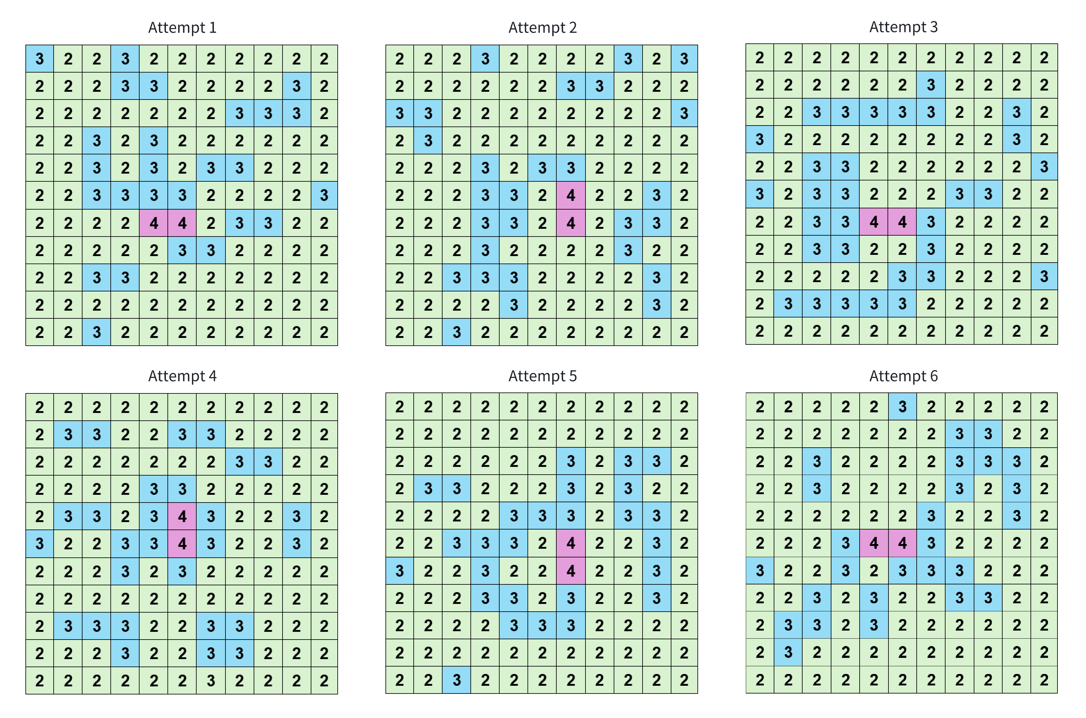
Figure 3 illustrates the neighbour distribution matrix result of six attempts to apply the improved Distribution Algorithm for generation. As can be seen, all the four patterns identified are present.
Improvements to the Braid Algorithm
In the original Braid Algorithm, the direction in which each iterated tile determines its neighbours is completely random. In order to achieve a better gameplay experience, it is also necessary to analyse the wall layout suitable for use as a PacMaze game map.
During the improvement of the Distribution Algorithm, Pattern 3 is discovered and summarised as “A tile with 3 neighbours is more likely to be adjacent to another tile with 3 neighbours at the same time.” By further observation of the classical map in Figure 1, a phenomenon based on this can be identified. That is, when a 3-neighbour tile has some adjacent 3-neighbour tiles, it has a big probability to actually become neighbours with these tiles. Therefore, the improvement idea that the Braid Algorithm can have when dealing with 3-neighbour tiles is, to favour the adjacent 3-neighbour tiles more, rather than depending on pure randomness.
Based on this idea, we can now design the logic that handles all 3-neighbour tiles in the improved Braid Algorithm. We first find all the 3-neighbour tiles from the list of all tiles on the map (shuffled). When processing each 3-neighbour tile, all adjacent tiles of that tile are stored, shuffled, and iterated one by one. Every time an adjacent tile is iterated:
- If it is a 2-neighbour tile, disconnect it with the current tile.
- If it is a 3- or 4-neighbour tile, it has a 90% probability to remain being neighbours with the current 3-neighbour tile. That is, it only has a 10% probability to be disconnected from the current tile.
The pseudocode of processing 3-neighbour tiles is as follows. Where the disconnect(), connect() and flood() methods are as defined in the original Braid Algorithm pseudocode by Ioannidis (2016). Note: the pseudocode in the original Braid Algorithm may be confusing disconnect() with connect(), since the logic of the algorithm should try to “build” a wall between two tiles first, and then “break” it if it is found that this is not fine.
1 | function handle_tiles_with_3_neighbours(all_tiles, current_neighbour_counts, distributed_neighbour_nums): |
In addition to this, another interesting phenomenon can be found by looking at the wall layout in Figure 1: the classic map has an apparent one-ring-over-one-ring phenomenon. Despite the fact that there are more 3-neighbour tiles in the inner rings, the presence of the rings can still be clearly observed. This makes the map visually more layered and makes it somewhat more difficult for Pacboy to avoid Ghostrons.
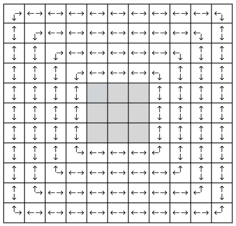
To ensure that the random map wall layouts generated by the improved Braid Algorithm follows this trend, some adjustment can be made to the neighbourhood preferences of all the 2-neighbour tiles in the map except for the central area, to help the generated map better present the one-ring-over-one-ring phenomenon. Figure 4 illustrates the most desirable neighbourhood scenarios for all 2-neighbour tiles of the map, except for the 3×3 area in the centre. For each tile location, its two arrows point to the directions in which its two neighbours would ideally be located.
Based on this idea, we can now design the logic that handles all 2-neighbour tiles not in the central 3×3 area, in the improved Braid Algorithm. We first find all the 2-neighbour tiles from the list of all tiles on the map (shuffled), that is not in the central 3×3 area. When processing each 2-neighbour tile, its neighbours are obtained and their order is shuffled. For each of all neighbours but two ideal neighbours of the current tile, it has a 85% probability to be disconnected the current 2-neighbour tile. That is, it only has a 15% probability to remain being neighbours with the current tile. If the number of neighbours of the current tile is still greater than its distributed value after traversing all non-ideal neighbours, its ideal neighbours are sacrificed.
The pseudocode of processing 2-neighbour tiles (not in the central 3×3 area) is as follows.
1 | function handle_non_centre_tiles_with_2_neighbours(all_tiles, current_neighbour_counts, distributed_neighbour_nums): |
Finally, we can deal with all the tiles in the central 3×3 area that are still not processed. Here, the same stochastic logic as in the original Braid Algorithm will be taken, so no pseudocode will be shown for this logic.
In summary, the whole logic of the improved Braid Algorithm is pseudo-coded as follows.
1 | function improved_braid_algorithm(): |
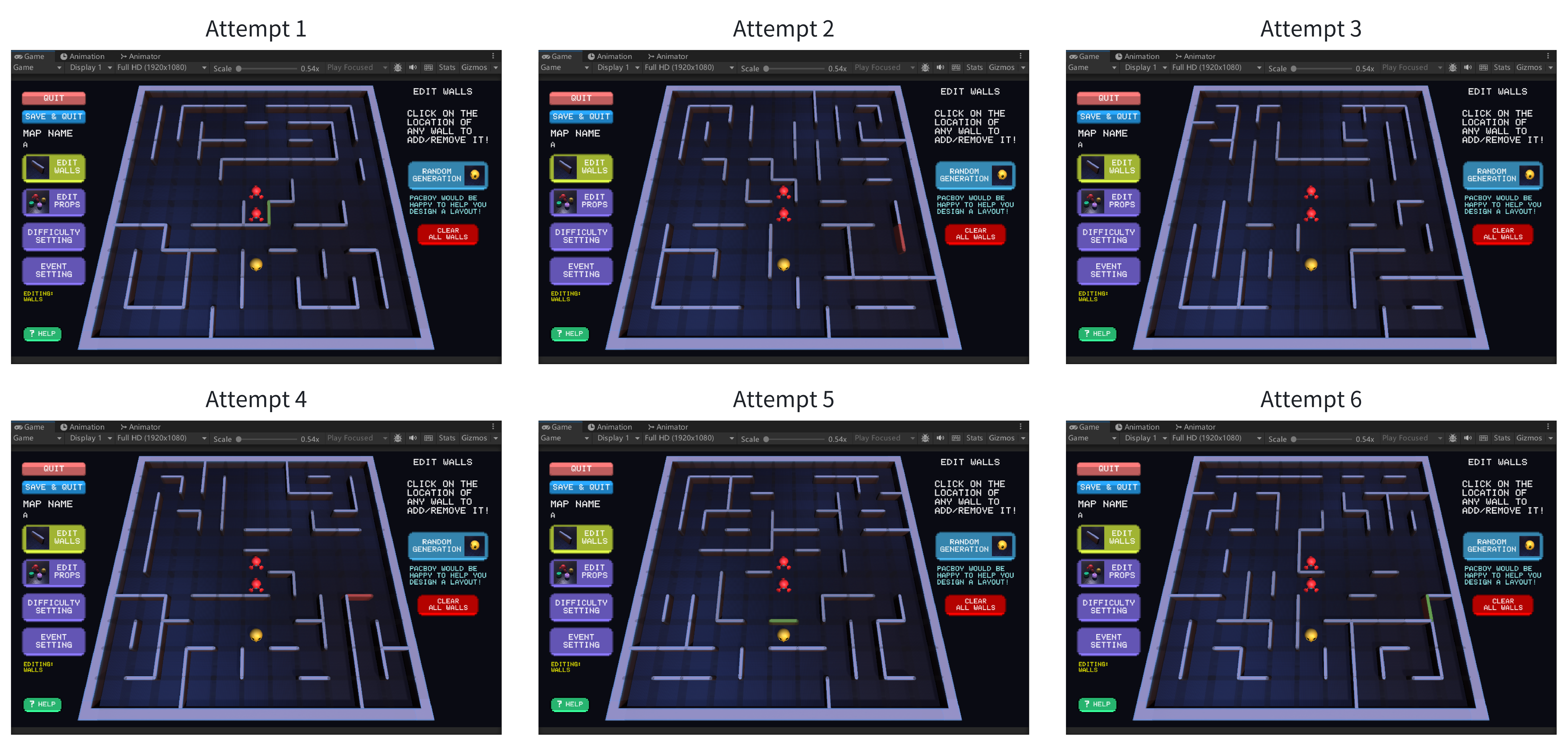
Figure 5 shows the result of six attempts to generate a map wall layout, applying the overall improved algorithm scheme.
References
This reference list is in Harvard style.
本引用列表采用 Harvard 风格。
Ioannidis P.L. (2016) Procedural Maze Generation. Bachelor Thesis. National and Kapodistrian University of Athens. Available at: https://pergamos.lib.uoa.gr/uoa/dl/object/1324569/file.pdf (Accessed: 6 May 2025).
Namco. (1980) Pac-Man [Video game]. Bandai Namco Entertainment, Arcade.
The graphic resources used in Figure 1 & 5:
图 1 以及图 5 中使用的图形资源:
https://assetstore.unity.com/packages/templates/tutorials/chomp-man-3d-game-kit-tutorial-174982
Unless otherwise stated, all posts from WaterCoFire are licensed under:
WaterCoFire 的所有内容分享除特别声明外,均采用本许可协议:
CC BY-NC-SA 4.0
Reprint with credit to this source.
转载请注明本来源,谢谢喵!